This is a total break from my usual paleontology content, but bear with me, because I think this topic is really interesting, fun, and useful.

Introduction to Bayes’s Theorem

The Reverend Thomas Bayes was a rather obscure 18th-century Presbyterian minister who made a single, ridiculously important contribution to mathematics: Bayes’s Theorem. This is a formula for calculating probabilities that takes into account prior knowledge, the things you already know or believe before you do the calculation. Statisticians who use Bayes’s Theorem for their probability are called Bayesians, while statisticians who don’t are called frequentists. Here’s a relevant xkcd highlighting the difference.

Bayes’s Theorem has important applications in machine learning, since it’s a way of formalizing the process of reasoning with uncertain information–essentially, getting computers to make good decisions even when they’re not totally sure about certain facts. The theorem is also culturally important in the rationality community, so much so that to many people, “Bayesian” is synonymous with “rationalist”.

Despite all the hype, Bayes’s Theorem is actually pretty easy to reason about and apply to various real-life problems. In this post, I’ll provide three examples of times I’ve used it in my own life, and hopefully by the end you’ll understand how to apply it to yours too.

Example 1: A Tea Party With Bayes

At work, in the before-time, we used have a tea party every Tuesday from 6 to 6:30. Before my company was bought by a larger company, it was a scotch party, where a bunch of middle-aged men would get together and taste the scotch of the week and try to guess what it was. But the larger company has a no-alcohol-on-the-premises policy, so it became a tea party. It’s kind of funny to see all these middle-aged men drinking tea and eating cookies and strawberries. It seems a lot more like an old-woman thing to do. Anyway, the game is that they’ll have some kind of plain tea–white, green, oolong, or black–and you have to guess which it is. If you’re really good, you’ll also guess what form (leaves, stems, powdered, etc) and what region (China, India, etc) and if you think it’s been served at the tea party in the past.

All this to say I realized I was making an un-Bayesian mistake when guessing tea. Let’s simplify it for now and just say there’s two kinds of tea, green and white. And let’s say my tasting skill is not that great yet, so I can distinguish between the two with a 60/40 success rate. So, 60% of green teas I taste will taste green to me, and 40% of green teas I’ll misidentify as white. Same thing with white tea: 60% I’ll correctly identify as white, and 40% I’ll wrongly guess green. One week, I tasted a tea, and it tasted white. So, stupidly, I guessed white. I was wrong. This is stupid because I disregarded my priors. White tea is way more rare than green, and I would estimate that for every white tea we have, we have nine green teas. So the prior probability of tea being white is 10%. Instead of shifting this probability when presented with new data, the 60/40 taste of it, I replaced my prior with the new number, and guessed it was 60% likely to be white tea. However, using Bayes’s equation, the true probability is only 14%, because there are so few white teas to begin with! Even if I could taste with 90% accuracy, the probability would only be 50% of being white tea. Let me explain the math:

• Out of 100 taste tests of tea, we can expect 90 of them to be green and 10 of them to be white. Easy so far.
• Out of the 90 green teas, there will be 54 that taste green (60% of 90) and 36 that taste white (40% of 90).
• Out of the 10 white teas, there will be 6 that taste white and 4 that taste green.

So, if I want to know the probability of a tea being white given that it tastes white (written mathematically as P(white | tastes white)) you do this:

\[P(\text{white} | \text{tastes white})=\frac{\text{number of white teas that taste white}}{\text{total number of teas that taste white}}\] \[P(\text{white} | \text{tastes white})=\frac{6}{6+36}=14.3\%\]

So you can see, the number of false positives I get from green teas that taste white is actually larger than the number of true positives, even though the false positives are a smaller proportion of the population.

Another way to visualize this calculation is to make a table:

	Tea tastes white	Tea tastes green
Tea is white	6	4
Tea is green	36	64

A presentation of data that shows the same relationships but looks different is called isomorphic. This table is isomorphic to the bullet points above.

Example 2: Taking Bayes On A Date

Here’s an example from a few years ago, when I was using Tinder, the speed-online-dating app. I was scoring each suitor in a spreadsheet on a few different categories, like “Musicality” and “Open-Mindedness” and “Attractiveness.” One time, I went on a date with a boy who got super high marks in all my predetermined categories; he was super smart, went to Harvard for undergrad and Oxford for grad, currently works at Facebook, knew a bit about rationality, had similar musical taste to me, was into climbing, played piano for 12 years, etc. Basically he was getting 7-9 in every category. But he seemed like he might be gay (and trying to date girls on Tinder because of familial pressure). Because of that, I added a new “other” category and scored him low on it, but he still came out with a higher score than any previous candidate. So then I decided to do a Bayesian calculation of how likely he was to be gay.

I’ve written about the fraternal birth order effect before in my post about strange biological phenomena related to pregnancy. For some reason, the more older brothers a right-handed man has, the more likely he is to be gay. For some strange reason, it doesn’t affect women and it doesn’t affect left-handed men. The prior probability of being gay (equivalent to the prevalence in the population) is about 3%. For every older brother you have, the probability goes up by 1/3.

STOP PRESS: I have since been informed that this equation is incorrect! See both my original derivation and the corrected equation in the Appendices to this post. However, this is what I used at the time, and this part isn’t part of the Bayesian calculation, so I’m leaving it as it was in this section.

The equation can be expressed as follows:

\[P_{gay}=1-\left(\frac{97}{100}\left(\frac{2}{3}\right)^n\right)\]

Where n is the number of older brothers. There’s an explanation of where this expression comes from at the end of this post, for those interested.

The suitor in question had one older brother. So, his prior probability of being gay was:

\[P_{gay}=1-\left(\frac{97}{100}\left(\frac{2}{3}\right)\right) = 35\%\]

I would guess that my gay-dar has an accuracy of 70/30. So, using this information along with the 35% prior probability, we can calculate

• Out of 1000 of this suitor,
• 350 will be gay and 650 will be straight.
• Of the 350 gay, 245 will seem gay and 105 will seem straight.
• Of the 650 straight, 455 will seem straight and 195 will seem gay. So the probability of him being gay given he seems gay is

\[P(\text{gay} | \text{seems gay}) = \frac{245}{245+195} = 56\%\]

So, even when taking into account the relatively small prior probability of being gay, I thought he was more likely to be gay than not, and I didn’t go on any more dates.

Again, we can represent the data isomorphically in a table:

	Seems gay	Seems straight
Is gay	245	105
Is straight	195	455

Being able to draw up a table becomes important when reasoning about more than two variables, as we’ll see in the next section.

Note: you probably have noticed that half of my Bayesian calculation each time comes from making up a number: my tea tasting accuracy of 60/40 and my gay-dar accuracy of 70/30. The point of doing a Bayesian calculation is that it makes you consider your priors and make a real statistical calculation, but once you get the result, you can make the choice to throw out the answer and go with your gut. But by doing this, your gut is much better informed.

Another interesting place the fraternal birth order thing comes into play is in the movie Frozen, in which Prince Hans says that he has twelve older brothers. If you’ve seen the movie, you know that he courts Anna just so he can gain control of her kingdom, so his sexuality isn’t really revealed by the story. Using the fraternal birth order calculation, we find that he has a 99.3% chance of being gay. Watsonianally, if Anna had known about the fraternal birth order effect, she could have saved herself a lot of trouble. Doylistically, I wonder if Disney’s writers knew about the fraternal birth order effect and intentionally invoked it when creating Hans’s backstory, appearance, and mannerisms.

Example 3: Bayes In The Time Of COVID

This example is from very recently, and is what inspired me to write this up as a post. Here’s what happened.

I wanted to visit my parents in person for New Year, so I got a COVID test even though I didn’t know of any particular exposures or have any symptoms. I had been going to work in person and had been to the doctor a couple times though, so I thought it would be prudent to get tested just in case. Surprise surprise, the test came back positive (if it didn’t, why would I be telling you this story?), so I cancelled my New Year plans and locked myself in a bedroom for ten days. However, I’d been living in the same house and sleeping in the same bed as my fiancé up until I received the test result, so for awhile we were worried that we would both get sick.

Thankfully, that didn’t happen: he tested negative twice (once maybe a bit early, but once in the theoretic peak detection time), and neither of us ever experienced any symptoms. That made me think, is it more likely that my result was a false positive, or that I truly had COVID but somehow didn’t transmit it to him? Time to bust out Bayes’s Theorem.

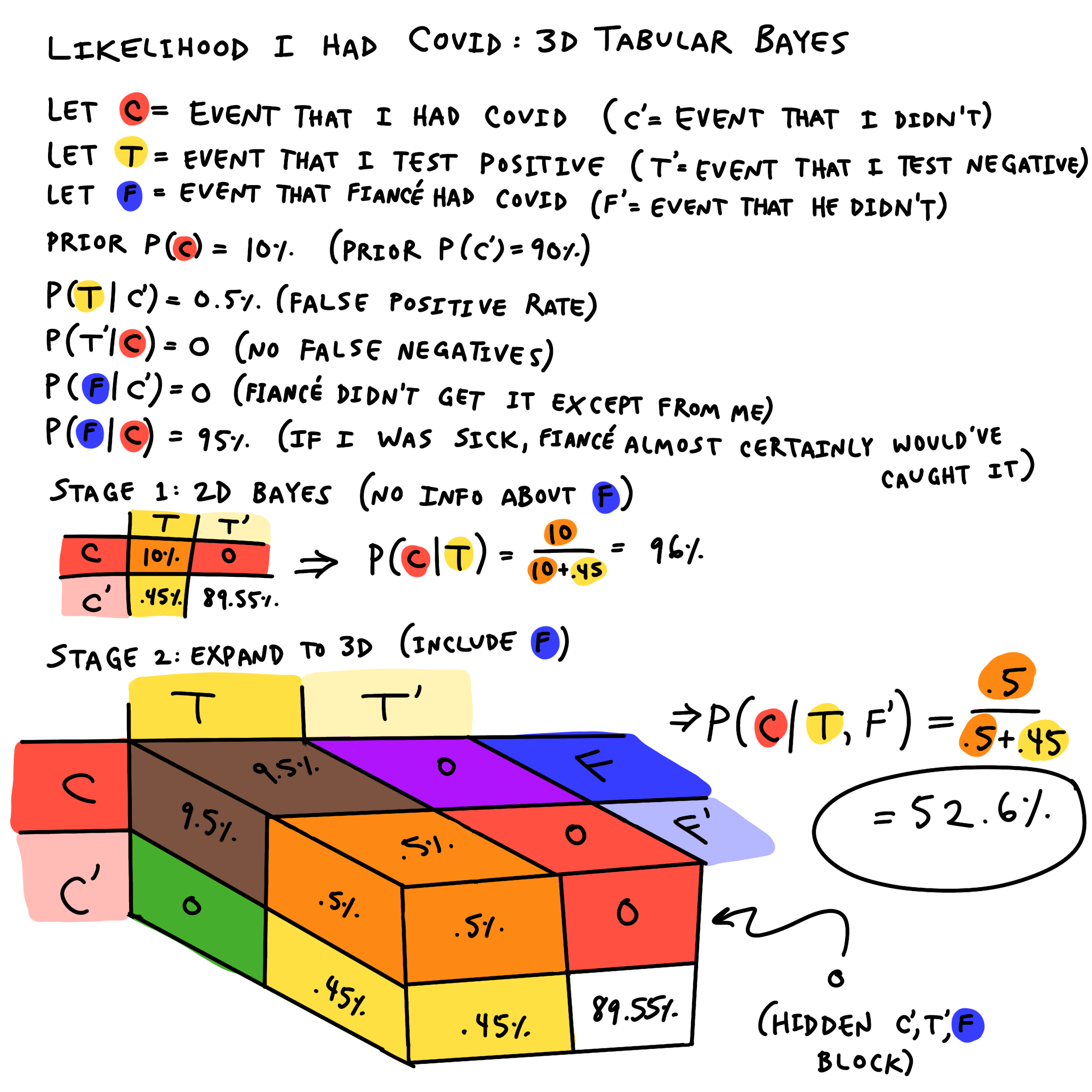
If you’re confident in your Bayes chops by now, feel free to just examine the graphic and skip this part. However, I’ll explain the process step by step here.

First, I define my variables. The ones with apostrophes are read “not-X” and are defined as one minus X. Straightforward so far.

Then, I state my priors and assumptions:

• My prior probability that I had COVID, before taking the test, was 10%–stated another way, I was 90% sure I did not have it. This is just my hand-wavey estimate.
• P(T | C’) = 0.5%: This is the false positive rate, which I looked up. There are a few studies on this, and most of them agree that 0.5%, or one in 200, is about right.
• P(T’ | C) = 0: I am assuming that there are no false negatives, meaning there are no cases in which I, a sick person, receive a negative COVID test result.
• P(F | C’) = 0: I am assuming that there is no way my fiancé could’ve gotten COVID except through me. This is reasonable because I was the only one who was going anywhere–he works from home, and we get groceries delivered.
• P(F | C) = 95%: This is the transmission rate, which I also estimated. Given we were essentially in the same room for the four straight days of peak contagiousness, the likelihood my fiancé would get COVID given I had it is very high. However, I’m not using 100% or even 99% because I think 95% confidence is pretty much as high as one should realistically bet on anything that isn’t a straight-up fact. (This is known as Cromwell’s Rule.)

Note: Since I’m assuming no false negatives (P(T’ | C) = 0), this also applies to my fiancé. That means P(fiancé does not have COVID) and P(fiancé tests negative) are equivalent.

Note also: The false negative rate on a single PCR-type COVID test is actually 20%, but in the United States they multiply the sample and run each test 40 times as part of the regular process, and if any single test comes back positive then the whole test is marked positive. That means the false negative rate is \(0.2^{40}=10^{-28}\) (that’s 0.00000000000000000000000000001) which is basically zero.

At this point I’m ready to create the usual two-variable table. Without knowing any information about the state of my fiancé, I went from being 90% confident I did not have COVID to 96% confident I did. This is due to the very low false-positive rate.

Now for the interesting new step: we expand the table in a third dimension, applying the conditional assumptions to “spread” the table’s probabilities across the new dimension. For many of them, the probabilities don’t spread at all: those are the cases I’m assuming have a probability of zero. However, one of them does spread–the 10% splits into a 9.5% block in the case of (C,T,F) and a 0.5% block in the case of (C,T,F’). That comes from applying the 95% transmission rate.

Finally, I can do the calculation:

\[P(C | T, F')=\frac{0.5}{0.5+0.45}=52.6\%\]

Wow, it’s quite a toss-up. Now I’m 52.6% confident (if you can call it “confident”) that I truly had COVID asymptomatically. Expanding the table again into 4D, using the probabilities of exhibiting symptoms given disease (P(S | C) = 40%, P(S | C’) = 0), is left as an exercise for the reader.

Appendix A: Correction to Fraternal Birth Order Effect Equation

A careful reader of this blog post did a little bit of their own research and discovered that the equation I used highly overestimated the power of the FBOE. I looked up the statistics of how many people in the general population have one older brother, two older brothers, etc, and used my equation along with this information to predict the proportion of gay men in the overall population. And that reader was right: my equation predicted that around 7% of men would be gay, when the actual value is 3%. I also cross-checked using the statement from the original paper that “15-28% of gay men can attribute their sexuality to the FBOE,” using those numbers along with the population’s prevalence of older brothers to generate an approximation of what the probability of being gay given one older brother would be, and came up with between 3.6 and 5.4%, not even close to the value my equation gives of 35%.

Why was I so wrong? I misinterpreted the authors’ statement of “increases by 33%” to refer to an absolute 33%, not a relative 33%. The correct interpretation was relative. Another way to put it: I thought it was 33% of 100%, but they meant 33% of the original probability.

So enough about me being totally wrong–what’s right? Well, the naïve interpretation of a relative increase of 33% every time could be expressed like this:

\[P_{gay}=\frac{3}{100}×1.33×1.33...\]

But eventually (between 12 and 13 older brothers) this probability exceeds 100%, which can’t be right–you know intuitively there should still be a small chance of having a straight son no matter how many sons you have. So clearly the “increases by 33%” trend can’t just continue exponentially. What’s a better model?

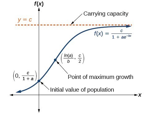
The logistic curve is a shape commonly found in population dynamics, and it handily looks very similar to exponential behavior for low values of n, but at some n it hits an inflection point and switches its behavior to logarithmic, asymptotically approaching a finite peak value. This is what it looks like:

The generalized equation for our logistic curve is written as follows:

\[P_{gay}(n)=\frac{1}{1+e^{-k(n-n_0)}}\]

Where k is a constant controlling the steepness of the growth, and n₀ is the n-coordinate of the inflection point. n is still number of older brothers.

Now, how do we solve for the constants k and n₀? We can plug in two known points, in this case P_gay(0) and P_gay(1). The former is equal to 3%, and for the latter we’ll apply “increases by 33%” just once to get 4%.

\[P_{gay}(0)=\frac{1}{1+e^{-k(0-n_0)}}=0.03\] \[\frac{1}{1+e^{kn_0}}=0.03\] \[e^{kn_0}=32.33\]

Now we can use this value of e^kn₀ when we plug in the value for P_gay(1):

\[P_{gay}(1)=\frac{1}{1+e^{-k(1-n_0)}}=0.04\] \[\frac{1}{1+e^{-k+kn_0}}=0.04\] \[1=0.04(1+e^{-k}e^{kn_0})\] \[k=0.298\] \[n_0=11.66\]

So the final equation becomes

\[P_{gay}(n)=\frac{1}{1+e^{-0.298(n-11.66)}}\]

Which looks like this:

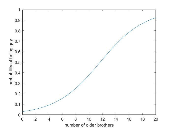
That’s a very differently shaped curve than the one I was using before! The probability doesn’t surpass 50% until you have 12 older brothers. Now I can redo my Bayesian calculation on that Tinder hopeful using the corrected prior of 4% for a guy with one older brother.

• Out of 1000 of this suitor,
• 40 will be gay and 960 will be straight.
• Of the 40 gay, 28 will seem gay and 12 will seem straight.
• Of the 960 straight, 672 will seem straight and 288 will seem gay. So the probability of him being gay given he seems gay is

\[P(\text{gay} | \text{seems gay}) = \frac{28}{28+288} = 8.9\%\]

Uh oh! I guess I should’ve gotten to know him a little bit better! Too late now.

Also, according to the new equation, Hans from Frozen (who does use his sword in his right hand) has a 52.5% chance of being gay, and Ron Weasley, who has five older brothers, has a 12% chance.

Thanks a lot to u/wupt on Reddit for correcting me! This logistic exercise was quite fun.

Original paper

Logistic curve image reference

Appendix B: Explanation of the Formal Expression of Bayes’s Theorem

If you look up Bayes’s Theorem, the most common way it’s expressed is

\[P(A | B)=\frac{P(B | A)P(A)}{P(B)}\]

We suspect this equation is just another isomorphism, but how do we get there from our intuitive tabular version?

Let’s go back to the tea example, because it’s simplest. Our final formulation of that problem was

\[P(\text{white} | \text{tastes white})=\frac{\text{number of white teas that taste white}}{\text{total number of teas that taste white}}\]

So in this case, “white” is event A, and “tastes white” is event B. The numerator, “number of white teas that taste white,” can be rewritten as

\[P(B | A)P(A)\]

because P(B | A) (probability of tea tasting white given that it is white) in the tea example is 60% (from our 60/40 statement of the problem), and P(A) is 10%, so P(B | A)P(A) = 6%, which we can see from the table is equivalent to “number of white teas that taste white”. In fact, that was how we generated that table entry–by first multiplying the total population by P(A) to get just the white teas, and then multiplying that portion by P(B | A), the 60% tasting accuracy. “Total number of teas that taste white” is equivalent to P(B). Despite its brevity, I think this is a rather unintuitive way of framing it, which is why I prefer the tabular version.

Appendix C: Derivation of My Original Incorrect Expression of Fraternal Birth Order Effect

This was how I derived the equation I used a few years ago when I was deciding whether or not to keep seeing that one suitor. Probabilistically, it’s still an internally consistent equation, but it doesn’t actually reflect the real fraternal birth order effect.

If you think about how probability “increases by 1/3” for every older brother, you might be tempted to just add probabilities like this:

\[P_{gay}=\frac{3}{100}+\frac{1}{3}+\frac{1}{3}...\]

But obviously at some point, it’s going to equal or exceed 100%, and you know intuitively that there’s still a chance of having a straight son even if you already have ten sons. So that can’t be right. Instead, you have to calculate the opposite–the probability of being straight–and subtract it from 100%. So, the probability of being straight is

\[P_{straight}=\left(1-\frac{3}{100}\right)\left(1-\frac{1}{3}\right)\left(1-\frac{1}{3}\right)...\]

which is equal to

\[P_{straight}=\frac{97}{100}\left(\frac{2}{3}\right)^n\]

where n is the number of older brothers you have. Now, sanity check, you can see that this probability will get smaller and smaller but will never equal or be less than zero. And the probability of being gay is one minus the probability of being straight, giving us the formulation

\[P_{gay}=1-\left(\frac{97}{100}\left(\frac{2}{3}\right)^n\right)\]